Theory Day 1

Several biological processes in the body generate electrical signals, that we can then detect using an electrode made of a conducting material (see Table 1 for an overview). We can record signals generated through skeletal muscle contraction (EMG), or heartbeat (ECG). In Neuroscience, we often use intracranial electrodes to measure action potential firing (spikes) or local field potentials (LFP). Electrodes outside the skull allow us to detect EEG non-invasively.

The methods for acquiring these signals have many things in common, which we will discuss during the upcoming week. We hope that you will learn to appreciate the broad similarities between these techniques, as well as understanding their differences, and what recording adjustments they require. When comparing different techniques, it’s important to understand:

1. What kind of signal do they measure?

2. What is a typical signal amplitude?

3. What kind of electrode (shape, material, size) is appropriate to use?

Introduction

Table 1; Overview of Extracellular Electrophysiology Methods

Technique	Signal	Electrodes	Typical amplitude
ECG/EKG	Heart: Depolarisation/repolarisation of cardiac tissue	Surface electrodes	mV range
EMG	Skeletal muscle: A train of motor unit action potentials.	Surface electrodes placed on skin above muscle, reference electrode on skin above bone.	mV range
EEG	Brain: Summations of neural activity	Surface electrodes on scalp	50 µV
LFP	Brain: Summations of neural activity	Intracranial electrode	100-1000 µV
‘Spike’ recording	Brain: Action potentials (‘spikes’) in individual neurons	Intracranial electrodes, e.g. tetrodes (4 insulated wires twisted together), Single-wire electrodes, Silicon probes.	20-200 µV

The first thing that all these electrophysiology techniques have in common is that the amplitude of the signals we are trying to measure is very small. Obien et al., (2015) gives us a direct comparison between the amplitude of an action potential measured inside the cell (measured in millivolts) and outside the cell (measured in microvolts). All electrophysiology techniques must detect tiny biological signals and convey them safely to a recording system (usually a computer) without losing or changing the signal.

To do that, they will need to:

1. Detect an electric potential difference.

2. Amplify this tiny signal.

3. Filter frequencies that are not of interest.

4. Digitize the signal for data visualisation and recording.

Most of the theory in this course will focus on intracranial extracellular recordings of neuronal activity, as these are the most common in systems neuroscience. For the practical exercises, we will be building an EMG recording circuit, as it is straightforward to test on yourself.

What are we measuring?

Neuronal electrical signalling is mediated by the flow of ions across the cell membrane, both into and out from the cell. These currents, whether at synaptic sites or during action potentials, can be measured as changes in the electric potential at a point in the extracellular space, compared to a reference point. This course will focus on how we get from tiny ion flows in the brain to a signal on our computer. First, we’ll go through a refresher on what these signals really are.

Charges and Current

Our biological signals are usually generated by ions, either positively charged (Na⁺, K⁺, Ca²⁺) or negatively charged (Cl^-). Electrons are the negatively charged particles in our electrodes and wires (i.e., metal) that allow these to conduct electrical signals. Charged particles exert a force on other charged particles.

\[F= k\frac{q1q2}{r^2}\]

Equation 1: F = electric force, k = Coulomb constant, q1 + q2 = charges, r = distance of separation.

Coulomb’s law (Eq 1) describes that this force will have both magnitude (depending on the size of the charges and the distance between them) and direction (it will either attract or repel, depending on whether the charges have the same polarity).

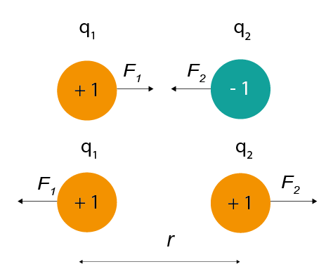
Figure 1: The magnitude of electric force between charges depends on their charge and the distance between them.

We often represent electric force with electric field lines surrounding the particle, to show that charges in the vicinity will be influenced by its force in a particular direction.

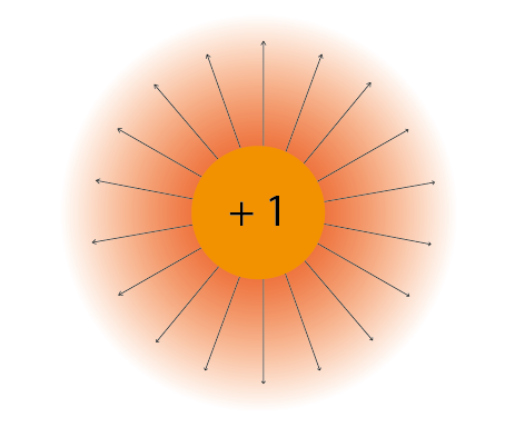
Figure 2: Electric field lines show the direction of the force on a positive charge. Colour intensity represents electric potential.

If a charged particle is free to move (for instance, it is in the cytoplasm, and not bound to a membrane) and placed within an electrical field, then these forces acting on it will cause it to flow in a certain direction, creating a current (I) measured in Ampere. The current tells us how much charge is moving per second.

\[I = \frac{Q}{t}\]

Equation 2: Current (I) is equal to charge (Q) over time (t).

By convention, the direction of this current is always the direction of positive charge movement. That means that when we talk about currents generated by a negatively charged ion, such as chloride, we describe it as a positive current moving in the opposite direction of the chloride ion.

Electric Potential Difference

Extracellular recordings measure the difference in electric potential (measured in Volts, and often called ‘voltage’) between two points. Electric potential is the ability to drive a current across a resistance; a recording of electric potential difference gives us a measure of the electric ‘pressure’ at one point compared to another. Just as a difference in gravitational potential energy can cause a river to flow down a mountain, a difference in electric potential can cause charged particles to flow from a region of higher potential towards a region of lower potential. The electric potential difference between two points tells us how much energy it would take to move a test charge from one point to the other. We are able to move a positive charge towards another positive charge, if we apply enough force in the opposite direction to overcome the repelling electric force. If we invest this energy and push our charges closer, we increase the difference in potential energy of the electric field at that location. If the charge is moved away, the potential energy decreases as it is converted to another form of energy, for instance to power a circuit. Figure 3 shows a negative and positive charge that are held in a certain position in space. They are not allowed to flow towards each other, but still exert an attracting force on each other. At any point in this space, the forces from the charges interact to give a net electric force that would be experienced by a positive +1 ‘test’ charge placed at that point. The vector description of the magnitude and direction of that force, is the electric field. In this figure, the electric potential is represented as height. The difference in electric potential between two points, tells us how much energy is needed to move from one to the other. A positive charge could easily ‘fall’ into the hole created by the negative charge. In contrast, we would need additional energy to push a positive charge up towards the positive peak, as we would have to counteract the repelling force generated by the positive point charge. If we add more point charges (that are not allowed to move) the generated forces will sum, giving a more complex map of electric potentials at every point in space. To describe the height of a mountain, there is no such thing as absolute altitude; instead, we use ‘sea level’ as our point 0 and measure from there. It doesn’t matter which point we take as point 0, as long as we use the same value when we are comparing measurements. The same goes for voltage: we pick a point to call ‘0 V’ and compare the rest of the circuit to that. This point can be the negative terminal of a battery, the extracellular fluid, or a point at infinity, far from all sources of electric potential (Einevoll et al., 2013).

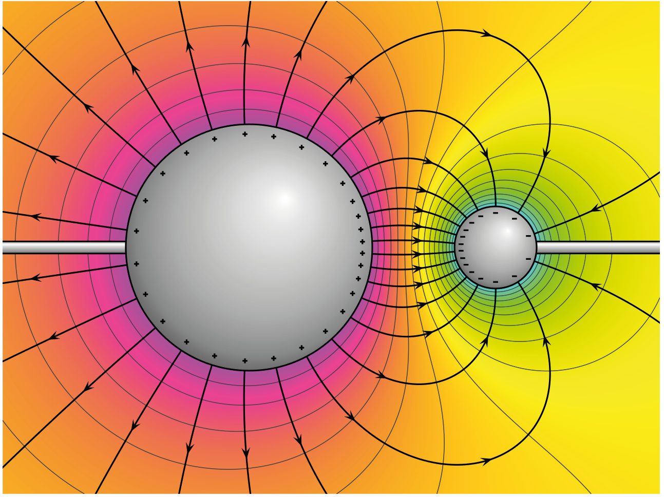
Figure 3: Electric potential mapped around a positive and negative charge.

© 2010 Geek3 /CC BY-SA 4.0, commons.wikimedia.org/wiki/File:VFPt_metal_balls_plusminus_potential%2Bcontour.svg

Neurons, Ions and Membrane Potential

Neuronal activity relies mainly on ions such as Na⁺, K⁺, Ca²⁺. Whenever these charges flow, we have a current. Resistance is a measurement of how difficult it is for current to flow. In neurons, the resistance to current flow is usually changed by opening or closing ion channels in the membrane. The more channels are open, the lower the resistance (to a certain ion), the more charge can flow in or out of the cell. As described above, the electric potential difference between two points tells us how much ability there is to drive a current between these points across a resistance. A neuron typically has a resting membrane potential of around -70 mV compared to the extracellular fluid, if we decide that the extracellular fluid has 0 V. This electric potential difference tells us that, to move a +1C charge from inside the neuron to outside the neuron, will require 70 mJ of energy. Indeed, neurons have to actively maintain their intracellular fluid at this lower potential with respect to extracellular space, by using ATP to power 3|Na+|/2|K+| pumps, which move Na⁺ out of the cell and reduce the amount of positive charge inside the cell.

Neuronal output: Action Potentials

When an input signal (a receptor potential or synaptic potential) depolarizes the cell membrane, this change in membrane electric potential can open Na⁺ ion channels. Na⁺ can then follow its concentration and electrical gradient from outside the cell, where the Na⁺ concentration is high, to the inside of the cell, where Na⁺ concentration is low and the intracellular medium has a lower potential (Kandel, Schwartz, & Jessel, 2000). In neurons, voltage-sensitive Na⁺ channels are usually concentrated at the initial segment of the axon, and it is therefore more likely that an action potential will be generated at the initial segment of the axon, rather than in other regions of the cell. The sudden influx of Na⁺ ions through these voltage sensitive channels in the cell membrane upsets the balance of processes that maintain the neuron at its resting equilibrium, and leads to a series of further changes which constitute the action potential (Hodgkin and Huxley, 1939). The extracellular potential Vec at position re, with respect to a point at infinity, can be computed with the following equation (Einevoll et al., 2013; Nunez and Srinivasan, 2006):

Equation 3: The point source equation.

Conceptually, this point-source equation (Equation 3) is key for computing the extracellular potential in response to any transmembrane current (Buzsaki et al., 2012). In(t) represents the nth point current source and re – rn represents the distance between the point source and the position of measurement, with n = 1…N, where N is the number of individual point sources and ρ is the extracellular conductivity. If the extracellular medium is considered homogeneous and isotropic, we can use a constant conductivity value (Einevoll et al., 2013).

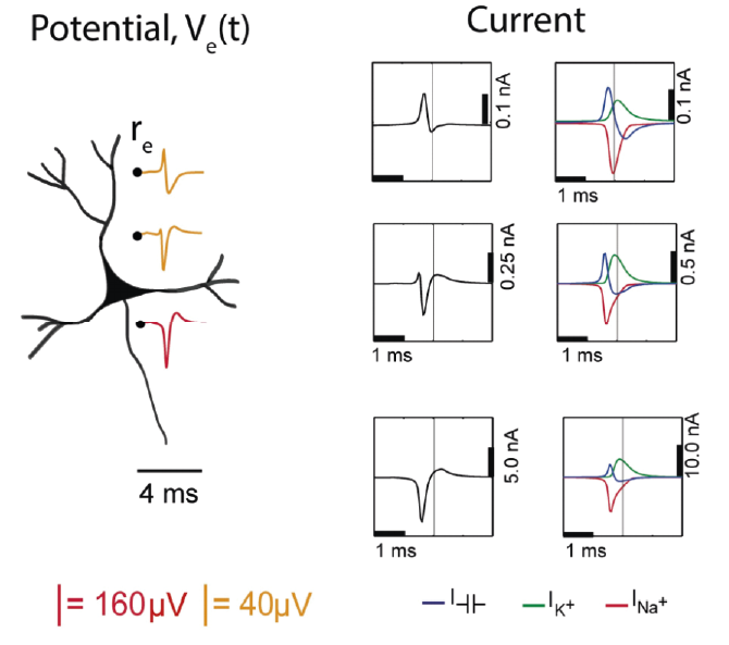
Figure 4: Electric potential generated by current sources in a conductive volume.

Electric potential generated by current sources in a conductive volume. The extracellular potentials and currents are adapted from Gold et al., 2006. Extracellular potential waveforms at selected spatial positions, re (marked with black dots) are simulated for a CA1 pyramidal neuron. Currents: simulated net membrane current (first column) across the soma and proximal dendrites that best estimates the extracellular potential waveform and membrane current components in terms of , |K+| and capacitive currents (second column). In the soma, the positive capacitive current coincides with the larger |Na+| current. At locations along the apical trunk, the initial capacitive peak becomes visible. In dendritic compartments the membrane depolarization is initially driven by |Na+| current from the soma, until local |Na+| currents are activated and the action potential regenerates. In the brief time before the local |Na+| currents activate, the positive capacitive current is the dominant membrane current and a capacitive-dominant phase is visible in the net current (Gold et al., 2006).

To detect the presence of an active neuron nearby in the extracellular space, the electric potential relative to some distant reference point must be measured. The model presented in Fig 4 illustrates how the electric potential varies nearby an active neuron. The extracellular potential waveforms usually last on the order of 1-2 ms, and are in the range of tens to hundreds of microvolts in amplitude, with the largest potential deflections being detected close to the soma of a neuron. These stereotypical temporal deflection of the electric potential in the extracellular space are called action potentials or spikes. Fig 4 depicts the time-varying extracellular potential at given locations (Re) that resulted from the superposition of the ionic and capacitive transmembrane currents formed when a neuron was active. The difference in potential waveforms at different locations in the extracellular medium is mainly given by the shape of the net current (Fig 4, left column) across the membrane. Furthermore, the peaks in the potential waveforms correspond to the current (Fig 4, right column) that is dominant at that time-point: the first positive peak of the waveform is attributed to the positive capacitive current resulting from the strong Na⁺ current entering the axon initial segment; the main negative peak is attributed to the influx of Na⁺; and finally, the second positive peak results from repolarizing K + current flowing out of the cell (Gold et al., 2006).

Neuronal input: Postsynaptic potentials

Slower frequencies in extracellular recordings are the focus of the LFP or EEG. These are thought to be largely generated by postsynaptic potentials, as these occur over slower timescales (10s of ms) than the action potential (1-2 ms), so there is more opportunity for signals from multiple cells to summate and result in larger signals. When activated, AMPA and NMDA synapses mediate excitatory currents as Na⁺ (AMPA) and Ca²⁺ (NMDA) enter the cell. This ‘sink’ of positive charge into the cell will induce a return current of positive charge (a ‘source’). Because of this, the direction of deflection caused by an excitatory current in an extracellular recording will depend on where the electrode is relative to the neuron.

The extracellular space

In the practical exercises for this course, we will be using electrodes attached to the skin. In animal models, we often use electrodes in the extracellular space. To keep things simple, most text book cartoons will draw neurons in the brain with a few synapses and lots of extracellular space in between each cell. If we were to stain all the dendrites and axons from every neuron in a slice of brain tissue, the result would be a solid black picture. A rat brain has about 200 million (and a human brain has about 86 billion) neurons tightly packed together (Herculano-Houzel, 2009). The density in the rat cortex is between 40,000 to 100,000 neurons per mm3 (Defelipe et al., 2002; Markram et al., 2015; Meyer and Moser, 2010). In addition to neuronal cell bodies, axonal fibres, and dendritic structures, the brain also contains glial cells and blood vessels. Very little of the extracellular space is actually “space”; indeed, extracellular fluid is thought to comprise only 12–25 % of the brain’s volume (Nelson et al., 2013; Tønnesen, Inavalli, & Nägerl, 2018). The potential Vec induced by the transmembrane currents depends on the magnitude, sign and location of the current sources, and on the conductivity of the extracellular medium (Buzsaki et al., 2012; Nunez and Srinivasan, 2006).

How do we measure these signals?

The acquisition system has to be able to:

1. Detect an electric potential difference.

2. Amplify this tiny signal.

3. Filter frequencies that are not of interest.

4. Digitize the signal for data visualisation and recording.

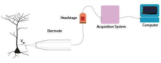
Figure 5: Components of an acquisition system.

The first step, detection, occurs at the interface between the biological sample or organism, and the electrode. Though the same ideas apply to all kinds of electrodes, here we’ll consider what occurs exactly when we record action potentials with a metal wire electrode. For now, we will simplify the rest of our recording system:

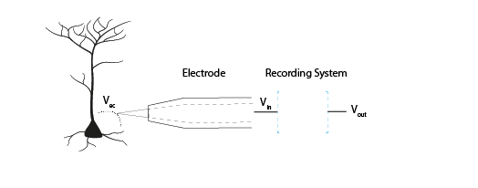
Figure 6: The goal of the acquisition system is to make the output voltage (Vout) as close to the extracellular voltage at the electrode tip (Vec).

We are interested in measuring the electric potential of the extracellular space (Vec) near a neuron. This must be relative to some point that we consider 0. In extracellular recordings, the recorded voltage (Vout) reflects the electrical potential difference measured between a microelectrode that is usually inside the brain, close to neurons, and the reference electrode somewhere else far from current sources in the extracellular fluid. Ideally, our Vec would be the same as our Vin (the input voltage to the recording system), which in turn would be the same as Vout. In reality we will always lose or distort some of the signal, but the challenge is to design our electrodes and recording systems to make Vout as close to Vec as possible.

Electrodes

Getting from neuronal activity (Vec) to the input to the recording system (Vin) relies first on the interface between the electrode and the extracellular space. Extracellular microelectrodes are usually made from metallic conductors. A thin insulated metal wire with an exposed tip is the most basic, and still widely used, device for in vivo extracellular recording from brains. Metals such as platinum, gold, tungsten, iridium, titanium nitride, stainless steel, iridium, iridium oxide, and alloys, nickel-chrome, platinum-iridium and platinum-tungsten have all been used in neural electrodes.

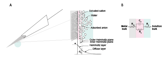
Figure 7: The double layer interface between an electrode and the extracellular fluid.

This transition from ion flow in the extracellular space (neural activity) to electron (electrode) flow is made through the double layer interface. When a metal is placed in a saline solution two phenomena occur: water dipoles close to the metal surface become oriented, and assuming the metal surface is negatively charged, the solution close to the metal surface become depleted of negative ions (anions), leaving behind a cloud of positive ions (cations). This cloud of cations screens the electric field caused by the excess of charge on the metal. Electroneutrality across the interface requires that the charge on the metal is always equal and opposite to the total charge on the solution side of the interface (Musa et al., 2012). The resulting charge distribution - two narrow regions of equal and opposite charge - is known as the electrical double layer (EDL). Figure 10 shows a model for the distribution of electric potential across a metal-solution interface, where the double layer region (represented in pink in the schematics) yields a capacitance Ce which typically has a value around 20 μF cm-2 (Musa, 2011). The signal transduction takes place across the electrode-extracellular space when the charge distribution changes on the extracellular fluid side. The electric potential variation in the extracellular space is accompanied by a redistribution of the ion concentration close to the metal electrode, and hence, changes in the electrode’s charges.

How does the electrode detect Vec?

Neuronal membranes have resistance- they are resistors. They also have capacitance, just as anything that is made up of two conducting layers, separated by a non-conducting layer, will have capacitance. We can extract the electrical behaviour of neural membranes and electrodes by making an ‘equivalent circuit’, which describes their electrical properties.

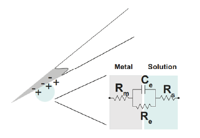
Figure 8: The equivalent circuit describes the electrical properties of the double-layer interface between electrode and extracellular fluid.

In the above figure, the interface between the solution and the electrode is represented by a parallel ReCe combination in series with resistances Rm (metal) and Rs (solution). • Re represents leakage resistance; the charge transfer due to charge carriers crossing the electrical double layer. • Ce is the capacitance of the electrical double layer at the interface of the exposed metal and the solution. Usually Re and Rs are small. For example, a tungsten microelectrode as the one used by Hubel and Wiesel in the 1950’s and 60’ has a value for Rm ~ 10 to 100 Ohm (Rm= (resistivity x length)/ cross sectional area), a Ce ~ 0.2 pF / um2 ~ 10 - 20 pF (unplated) and Re ~ 10 to 100 MOhm. This microelectrode is considered a ‘polarized’ electrode. There are two general types of electrode, ‘non-polarised’ and ‘polarized’. Each has a different mechanism through which ion flow in the solution leads to electron flow in the electrode.

Non-polarized electrodes

The well-known silver-silver chloride (Ag-AgCl) electrode approaches the ideal nonpolarizable type. In these ‘charge transfer’ electrodes, surface-confined species are oxidized and reduced (Bard & Faulkner, 2001, Merrill et al., 2005). Non-polarizable electrodes have a small Re, allowing charge-transfer across the electrode-solution interface. If Re is small, it bypasses the capacitor Ce, thus providing a DC path for the measurement of steady potential levels.

Polarized electrodes

Alternatively, the transition from ion flow in the solution to electron flow in the electrode could be of capacitive nature, involving the charging and discharging of the electrode-solution double layer. This happens with noble metal (e.g., stainless steel, gold and platinum) electrodes, where no charge transfer can occur across the metal-solution interface. Instead, electrode polarization is required to motivate current flow in the external recording circuit. In metals, such as aluminium and copper, charge transfer occurs and causes metal’s deterioration (i.e., oxidation). The value of Re of polarized electrodes is large, in the order of several megohms, and the effective equivalent circuit is dominated by the capacitor, Ce. Therefore, processes in polarizable electrodes are purely electrostatic and caused by the charging and discharging of the double layer capacitance. Although charge does not cross the interface, external currents can flow when the potential or solution composition changes (Cooper, 1971).

Acknowledgements

Written by:

• Alexandra Leighton

• Joana Neto

• Jakob Voigts

• Aarón Cuevas López

• Jon Newman

With material from:

• Joana Neto, 2018; Materials and neuroscience: validating tools for large-scale, high-density neural recording, 2018.

• Jon Newman and Jakob Voigts, 2017; Intro to Chronic Ephys (presentation at TENSS)

• Mitra Javadzadeh, 2017; Building an analog ephys recording system (practical exercises developed for TENSS)

Licensing

This work is licensed under CC BY-SA 4.0. To view a copy of this license, visit https://creativecommons.org/licenses/by-sa/4.0/

References

Bard, A. J., & Faulkner, L. R. (2001). Electrochemical methods Fundamentals and Applications. Molecular Biology (Second, Vol. 8). John Wiley & Sons, Inc. http://doi.org/10.1016/B978- 0-08-098353-0.00003-8

Buzsaki, G., Anastassiou, C.A., and Koch, C. (2012). The origin of extracellular fields and currents - EEG, ECoG, LFP and spikes. Nat Rev Neurosci 13, 407–420.

Defelipe, J., Alonso-Nanclares, L., and Arellano, J. (2002). Microstructure of the neocortex: Comparative aspects. Journal of Neurocytology 31, 299–316.

Einevoll, G.T., Kayser, C., Logothetis, N.K., and Panzeri, S. (2013). Modelling and analysis of local field potentials for studying the function of cortical circuits. Nature Reviews Neuroscience 14, 770–785.

Gold, C., Henze, D.A., Koch, C., and Buzsáki, G. (2006). On the Origin of the Extracellular Action Potential Waveform: A Modeling Study. Journal of Neurophysiology 95, 3113–3128.

Herculano-Houzel, S. (2009). The human brain in numbers: a linearly scaled-up primate brain. Front. Hum. Neurosci. 3.

Hodgkin, A.L., and Huxley, A.F. (1939). Action Potentials Recorded from Inside a Nerve Fibre. Nature 144, 710–711.

Kandel, E.R., Schwartz, J.H., and Jessel, T.M. (1991). Principles of neural science.

Markram, H., Muller, E., Ramaswamy, S., Reimann, M.W., Abdellah, M., Sanchez, C.A., Ailamaki, A., Alonso-Nanclares, L., Antille, N., Arsever, S., et al. (2015). Reconstruction and Simulation of Neocortical Microcircuitry. Cell 163, 456–492.

Merrill, D.R., Bikson, M., and Jefferys, J.G.R. (2005). Electrical stimulation of excitable tissue: design of efficacious and safe protocols. Journal of Neuroscience Methods 141, 171–198.

Meyer, A.C., and Moser, T. (2010). Structure and function of cochlear afferent innervation. Curr Opin Otolaryngol Head Neck Surg 18, 441–446.

Musa, R. (2011). Design, fabrication and characterization of a neural probe for deep brain stimulation and recording.

Musa, S., Rand, D.R., Cott, D.J., Loo, J., Bartic, C., Eberle, W., Nuttin, B., and Borghs, G. (2012). Bottom-Up SiO2 Embedded Carbon Nanotube Electrodes with Superior Performance for Integration in Implantable Neural Microsystems. ACS Nano 6, 4615–4628.

Nelson, M.J., Bosch, C., Venance, L., and Pouget, P. (2013). Microscale Inhomogeneity of Brain Tissue Distorts Electrical Signal Propagation. J. Neurosci. 33, 2821–2827.

Nunez, P.L., and Srinivasan, R. (2006). Electric fields of the brain: the neurophysics of EEG (Oxford ; New York: Oxford University Press).

Obien, M.E.J., Deligkaris, K., Bullmann, T., Bakkum, D.J., and Frey, U. (2015). Revealing neuronal function through microelectrode array recordings. Front. Neurosci. 8.

Ray Cooper. (1971). Recording Changes in Electrical Properties in the Brain in Methods of Psychobiology. (R. D. Myers, Ed.) (Volume 1). London and New York: Academic Press.

Software Requirements Exercises Day 1